Mathematics Section ℼ
The language of our universe
Mathematics is one of the most important fields of study in the world; it can be found everywhere from Physics, Finance, Biology, Geography, Architecture, Psychology, Music, Art, and literally any field you can think of. Every great achievement in human life has some mathematics behind it.
It is also found everywhere in nature, from the geometrical shapes of every living and non-living thing that all seem to follow consistent rules, to the symmetrical relationships of many natural objects, and the beautiful and pleasing patterns we hear in music. Whether we see it or not, mathematics is everywhere. Mathematics is the one subject that seems to connect different fields that seem barely connected. I am a firm advocate of Galileo's quote of “Mathematics is the language with which God has written the Universe!”. As such, I believe the more we understand mathematics as people, the more we begin to understand the world.

As we all know, mathematics is one of the most disliked subjects by people, mostly due to the way they were taught in schools and because many people believe they are not very good at it. But personally, I don’t think you need to be good with equations and all those other things to truly appreciate mathematics, as it is a lot more than just numbers and equations. In this section, I try my best to show anyone reading this the beauty of mathematics, to gain a better appreciation of it. Please do not be intimidated by the equations, I tried my best to write them in a way that it still makes sense even if you ignore them.
As of now, this is still a work in progress; mathematics has so much to offer, so I will add more things as time goes on. I hope you enjoy and maybe learn something.
i. Mathematics and Psychology
Last edited on August 2024
Weber -Fechner laws in psychometrics
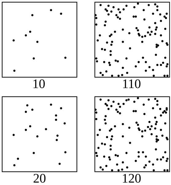
If you are carrying 100 books and someone adds 1 book to your load, you probably wouldn't notice the difference vs if you were carrying just one book, right? That's what the Weber-Fechner laws tell us regarding stimulus as a whole. The Weber law says in order for us to tell the difference, there has to be a 2% change in the stimulus, for example if there's 10 spoons of sugar in a cup of tea, you have to add 0.2 of a spoon to feel any change, if there is 100 however, you have to add 2 spoons, if you add one you won't feel a difference according to the theory. It accounts for all other sensations as well: hearing, seeing, smelling, and touching.
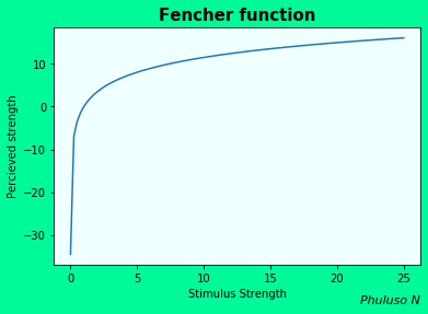
Then there's the Fechner method, which says there's a logarithmic relationship between the perceived strength and the stimulus strength, hence the change in perceived stimulus declines the stronger a stimulus gets, since the derivative(\(dy\over dx\)) of \(y=log(x)\) is declining for positive values, kind of like diminishing marginal utility. Economists have also used these theories to study some consumer behaviour.
The exponential model of memory retention
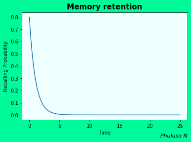
According to many psychologists, the ability to retain what you just learned declines quickly at first, then levels off as time passes. According to a Wixted and Besen study of 1991, it can be represented by an exponential model p= \(aex^{-bx}\), where p is the probability of a person being able to correctly recall an item learned. \(x\) is the time since learning it. And 0< a< 1 being the baseline retention before time passed, b>0 is the rate of retention drops with time, if your b is lower, your probability of retention drops at a lower rate. So don't start studying the day before your exams, basically.
ii. Mathematics and Love
Last edited on September 2024
If you were to ask someone about the relationship between maths and love, they'd probably tell you about how much they hate it…(I swear the joke sounded better in my head). Anyway…:
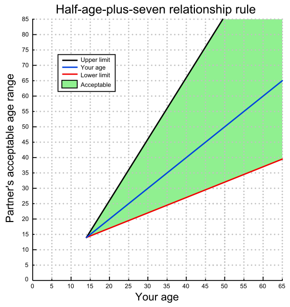
There's a formula for the socially acceptable dating age difference between men, and women and it is \({Age\over 2}\)+7. So, if a person is 30, the youngest person they should date is \({30\over 2}\)+7=15+7=22. The formula is a y=mx+c type graph hence the acceptable age difference keeps rising the older the 2 people are, as you can see from the graph.
Apparently, this formula has been around since the early 1900s; however, it was not meant to be for the youngest age a person should date, like it's used today, but the ideal age of a partner for a man, which is interesting. Studies have shown it's fairly accurate, but only when the man is the older person. According to a USA study from 2017, a huge majority of married couples in the US have an age gap of 1-3, and that is more common in many other countries too.
The Mathematics of Marital Conflict, 1998 study by John Gottman, Catherine Swanson, and James Murray.
50% of married American couples end in divorce, and some researchers did a study on why this happens by putting couples together and letting them talk while they analysed their conversations, facial expressions, and many other factors and then made a mathematical model that predicts whether or not they’d end in divorce.
-
Summary of the process
-
Analysis of the graphs
-
Conclusions from the findings
They computed for each conversation turn. Behaviour was considered positive if it correlated positively with marital happiness and negative otherwise. The Rapid couples interaction scoring system (RCISS) and the Specific Affect Coding System (SPAFF) was used to create numerical values of the behaviours. The sequence of scores were \(W_t\,H_t,W_{t+1},H_{t+1}\).\(H_t\) is the husband variable at time t, and \(W_t\) is for the wife (so it's: wife talks, husband responds, wife responds, and so on.)
$$ W_{t+1}=a+r_1W_{t}+I_{HW}(H_t) ... (1) $$ $$ H_{t+1}=a+r_2H_{t+1}+I_{WH}(W_t) ... (2) $$
\(a\), \(b\) and \(r\) are the parameters estimated from the data. \(r\) is the emotional inertia, which is the tendency of the person to remain in the same state over a period of time. \(a\) and \(b\) is the initial uninfluenced level of positivity minus negativity each spouse brings to the interaction. The \(I_{HW}\) and \(I_{WH}\) are the influence functions. Once the \(r_1\),\(r_2\), \(a\) and \(b\) are estimated from the data, (\(a\)+\(r_1W_t\)) and (\(b\)+\(r_2H_t\)) are then subtracted from equations (1) and (2) respectively, and the remainder will be the influence functions which were then plotted.
There are 2 types of graphs for both husband and wife (one type is for a couple that ends in divorce and one type is for a couple that has a lasting marriage), but we'll focus on the 2 types of husbands in a couple since the graphs are the same for the wives.
Graphs A and B represent the influence the husbands have on their wives; what the husband does is the x-axis, and the wife's reaction is the y-axis. In graph A, the husband has no influence on her until he does or says something at P or -P, then he gets either a big positive or a big negative reaction. And in B, the husband in a different couple, gets a little reaction for everything he does, either positive or negative, so the growth is linear. Before we move on, in your opinion, what couple do you think would have a longer lasting marriage?
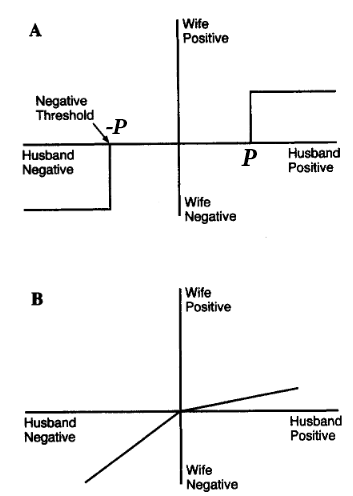
They used the term “threshold of negativity” , which is the point at which negativity has an impact on the partners immediately following the behaviour. Apparently, a low threshold like in B, means couples end up happy and stable. It is the "negativity detection effect", spouses responding to negative behaviour when it is less escalated.
With a couple of graph A, they accept negativity. Setting their threshold for a response at a higher level or more negative level, then blowing up when they've had enough, if the negativity threshold is really high, it means either the husband or wife has to become very aggressive to get a proper reaction from their spouse in an argument, which is a high risk factor for divorce, meanwhile couples in graph B who see a problem and immediately bring it up before it escalates too high usually have a longer lasting marriage, it was compared to how it's better to go to the hospital immediately when you notice a symptom and not when a disease gets worse. The bible verse Ephesians 4:26 ‘’Do not let the sun go down while you are still angry’’; was stated to support this. On the contrary, though some studies have suggested that couples can cultivate an empathetic response to their partner's negativity, but they didn't say anything about that leading to a longer lasting marriage.
iii. Mathematics and Medicine
Last edited on August 2024
Computed Tomography

Computed Tomography scanning, commonly known as CT scanning, is a radiographic imaging technique that generates cross-sectional images of organs and tissue structures. An X-ray tube rotates, scans, and performs measurements from different angles, which is then sent to a computer that does a mathematical algorithm and solves a certain integral, then gives results. It is used for diagnosing patients and with checkups. Maths used includes the Radon and the Fourier transform, Fourier slice theorem, some numerical methods, and other mathematical techniques.
iv. Mathematics and Geography
Last edited on August 2024
Global positioning system
The Global Positioning System , also known as GPS, helps solve the main problem of navigation with maps, which is where you are on the map. It uses trilateration, which is based on measuring distances using geometry and trigonometry. Satellites transmit radio signals containing the time the signal was sent and the location of the satellite, the signals are then received by GPS receivers like our phones. Since the electromagnetic waves travel at the speed of light, they arrive after a certain time duration. We find the distance by multiplying the speed of light and the time it took the signal to arrive \(distance={speed\times{ (received\space time-sent\space time)}}\). Then spherical geometry and 2 other satellites are used to find the position of the GPS.
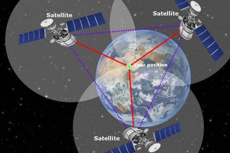
4 satellites are actually needed because there's a time offset between our phones and the atomic clocks used by satellites. So, a 4th satellite and some calculus are used to calculate the offset time. Satellites are placed in a way that we can access at least 4 from wherever we are, which is pretty cool. Einstein's theory of relativity also plays a factor since satellites orbit the earth at really fast speeds and experience less of the earth's gravity, which affects their atomic clocks. These conditions are, however, integrated to the computers that do these calculations, thus accounting for the rates of the atomic clocks. If this wasn't done, there'd be an added error of 10km every day, which is crazy to think about. Mathematicians, engineers, and scientists are the real unappreciated heroes of our modern world, honestly.
v. Mathematics and Politics
Last edited on August 2024
Median Voter Theorem
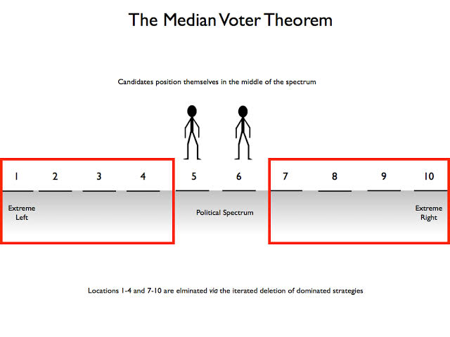
the median voter theorem states that political parties that cater to the median or average person in a group of people are more likely to win, because if for example a party tries to cater too much to the rich people they might lose voters from the poorer group and if they cater to the poor they'll lose votes from the rich, but if they cater to the middle persons though they'll get votes from middle people, some votes from rich people and some from the poor who are willing to compromise vs a party that only caters to and gets votes from one side. It's not just rich and poor that play a factor in who the middle person is, but also a wider range of ideologies and/or policies. I learnt about this little theory in second year economics, and it also applies to businesses too, sometimes even movies. The model has some obvious flaws, which I won't delve into, but you can go and learn more about it if you're interested.
vi. Mathematics and Economics
vii. Mathematics and Music
viii. Mathematics and Art New
Last edited on January 2026
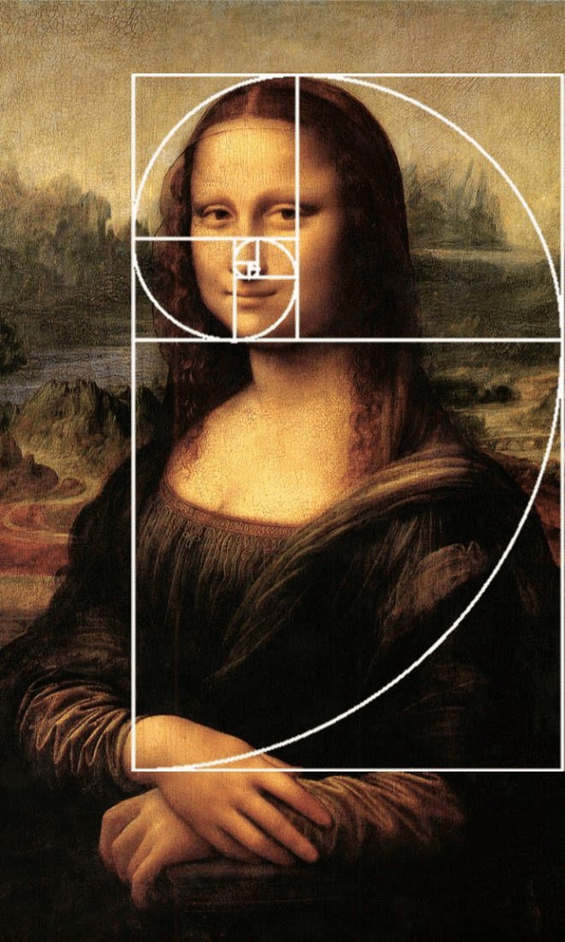
The golden ratio
The golden ratio, also known as the divine proportion, in simple terms, is a ratio between 2 numbers which is an irrational number approximately equal to 1.618, denoted by \(\phi\). But where does the number 1.618 come from?
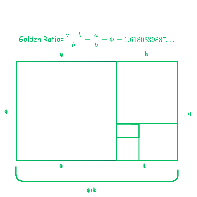
Suppose we have a rectangle with dimensions \((a+b)\times a\), then we draw another rectangle of the same proportion and same length as the previous rectangle inside said rectangle, then we have another rectangle of dimensions \(a\times a\), We can keep repeating the process to infinity, but for now let’s focus on the first 2 rectangles. The ratios of the 2 rectangles will be: $${{a+b}\over a}={{a}\over b}=\phi$$ $$1+{{a}\over b}=1+{{1}\over \phi}$$ $$1+{{1}\over \phi}=\phi$$ $$\therefore \phi^2-\phi-1=0$$ and using the quadratic equation we get: \(\phi\)=\({1+\sqrt{5} }\over 2\)=\(1.6180339887...\)
Relationship between the Fibonacci and the Golden ratio.
Before we get into the relationship between the Fibonacci sequence and the Golden ratio, let's talk about the Fibonacci sequence. What is the Fibonacci sequence?
The Fibonacci sequence is a recursive sequence where each number is the sum of the two previous numbers in the series. For example, look at the first 10 terms of the sequence: $$ 0, 1, 1, 2, 3, 5, 8, 13, 21, 34... $$ Notice how 8=5+3(the 2 numbers before 8),13=8+5(the 2 numbers before13) and so on. This can be mathematically recursively defined as: $$ F_0=0\\ F_1=1\\ F_{n}=F_{n-1}+F_{n-2}\ (where\ n\ \in\mathbb{N} ,n\geq2)$$ and also, non-recursively defined as $$F(n) = { 1\over {\sqrt5}}\Biggr[({1+\sqrt{5} \over 2})^n-({1-\sqrt{5} \over 2})^n\Biggr](where\ n\ \in\mathbb{N})$$ The second formula is obtained by applying the first formula in conjunction with the power series and performing some algebraic manipulations, which I will not elaborate on here. Back to the first 10 terms of the Fibonacci shown above, notice how \(13 \over8\)=1.625, \(21 \over13\)=1.615, and \(34 \over21\)=1.619? The ratios between the 2 consecutive numbers of the Fibonacci sequence converge to the golden ratio \(\phi\) the bigger the Fibonacci sequence grows in mathematical terms: $$ \lim_{n \to \infty}{F_{n}\over F_{n-1}}= { {1+\sqrt{5} }\over 2}=1.6180339887...$$
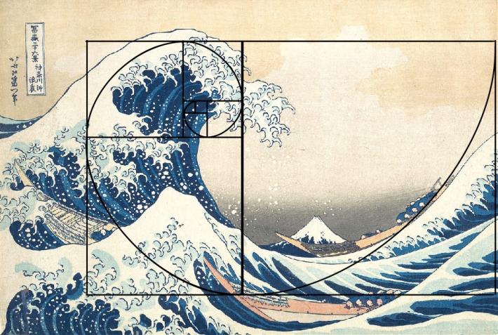
The golden ratio and beauty:
The golden ratio has been observed to appear in numerous places in nature and is considered visually pleasing by many. As a result, artists over the years have sought to incorporate this beauty by applying the golden ratio in their artworks.

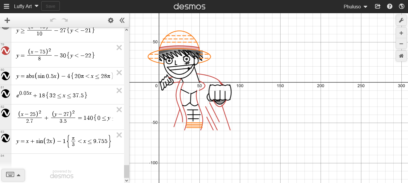
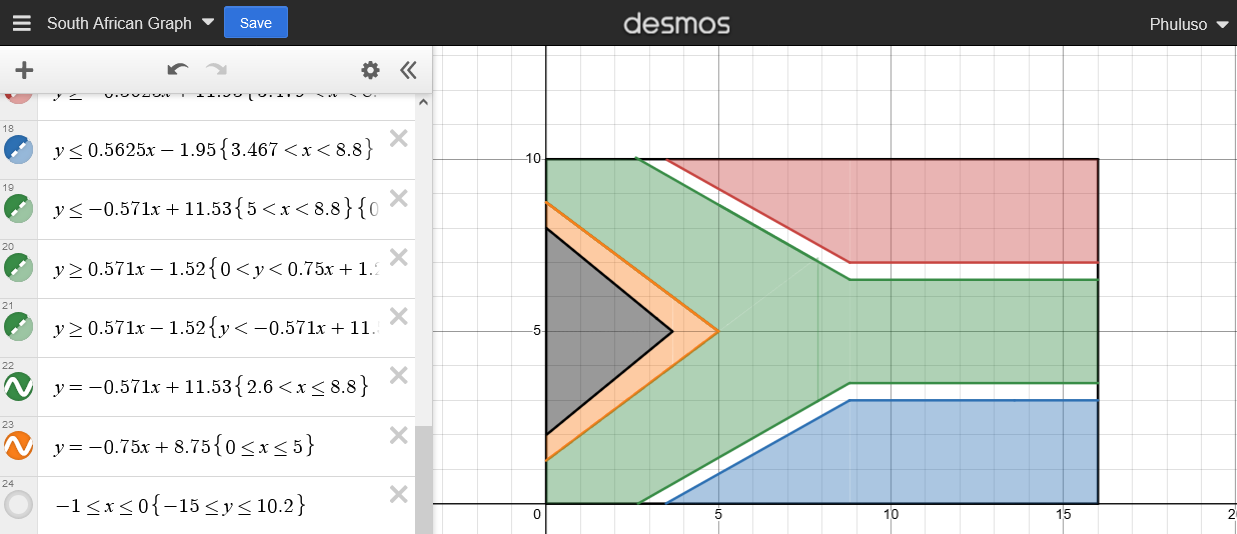
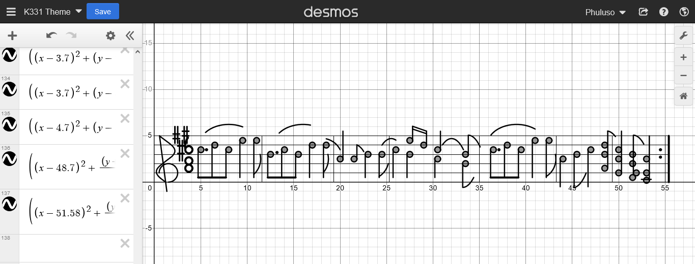
My Graph Art
These are some of the artworks I’ve made using the online graphing calculator Desmos. Not the greatest pieces of Desmos art ever created, but I had a lot of fun making them, and I am very proud of them.
Convergence and Equilibrium
Last edited on August 2024
Convergence
Convergence and equilibrium are 2 of my favourite concepts in mathematics; they are both cool concepts which can be found anywhere and are the backbone of our modern world. Now, without further ado, let's start off with convergence. What is convergence? Convergence is when things from different places meet at a point or place.
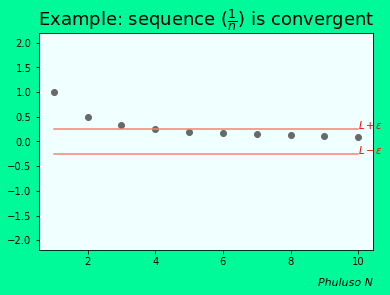
In mathematics, you see this with sequences and functions as they approach a limit; a convergent function/sequence will just keep getting closer and closer to the convergent point as the domain values increase or decrease. This is a formal mathematical definition of convergence:
A sequence \(a_{n}\) converges to limit \(L\) if and only if for every \( \varepsilon > 0 \) there exists a natural number \(N\) such that \(\forall_{n\epsilon N}\) :$$n >N \Longrightarrow \ |a_n-L|<\epsilon$$ this is denoted by \(lim_{n \rightarrow \infty }a_n=L\).\(a_{n}\) tends to \(L\) as \(n\) tends to infinity, which basically describes what is happening in the following graph
One thing that makes mathematical convergence possible is limits in calculus, because they help us make use of the concept of infinity. Limits and convergence are the backbone of numerical analysis. Numerical analysis helps us solve problems that are unsolvable by conventional means, by using approximations that are so close to the answer they're practically the same as the answer. Numerical methods include the Gauss elimination method, the Taylor series (which can approximate any function as a polynomial), the Riemann sum(for integrals), the Finite difference method (for differential equations), the Newton-Raphson method, the Euler method, Runge-Kutta methods, the Gradient descent, and many others.
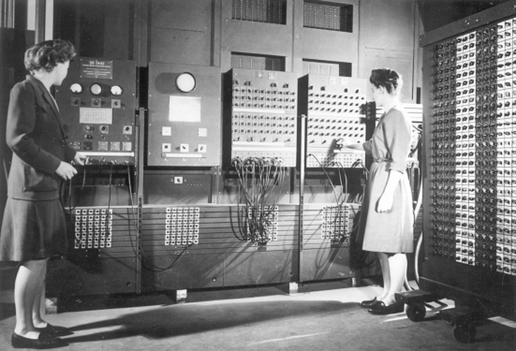
Since these methods are algorithmic, they require a lot of iterations to get accurate results, but thanks to computers, this is made easier. Computers are particularly very good at equations like these if programmed correctly. Back in 1943-1946, the ENIAC(Electronic Numerical Integrator and Computer) was developed. It was built to solve numerical problems(among other things ) to help with the war and calculate ballistic firing tables quickly. The ENIAC could do 5000 calculations per second; smartphones nowadays can do more than 100 billion calculations per second.
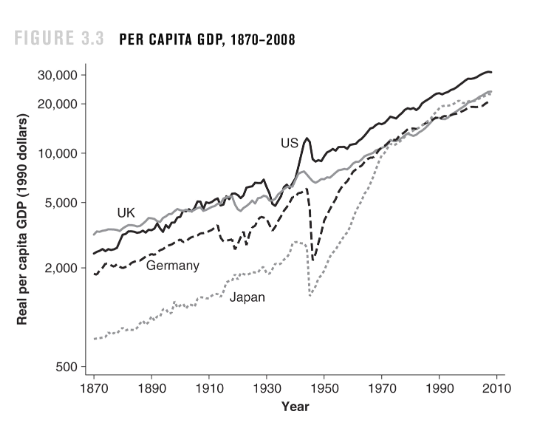
Convergence is useful in many branches of mathematics, like statistics and probability, with the Central limit theorem and the law of large numbers, which states that the larger the sample, the more the results converge to the true value. It's also useful in computer science and machine learning with the gradient descent algorithm. In Economics there is a theory that states that poor countries converge to richer countries. Developing countries have the potential to grow at a faster rate than developed countries because of diminishing marginal returns. Rich countries have already developed their science and technologies, so poor countries can learn just from them, right? Well…that’s not always the case for a variety of reasons, but we’re talking about convergence, not economics! (Image source: Introduction to Economic Growth, 3rd Edition. Norton & Company.)
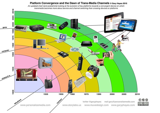
There's a lot more convergence phenomena in our world, like convergence in animal evolution, where some animals have developed similar traits despite having no common ancestor with that specific trait. E.g., butterflies, birds, and bats both have wings but no common ancestor with wings, maybe pigs will really fly someday, who knows. There is also Media convergence, which is the process by which multiple media technologies are brought together into one computerised device.
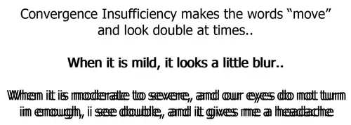
Another one is Convergence insufficiency, which happens when the nerves that control our eye muscles don't work the right way. Which means in the absence of convergent insufficiency, our eyes are always converging when we look at things.
There is also convergence in research, where a development in one research field leads to a development in many other fields.
As you can see, Convergence is everywhere!!! Are there any other convergence phenomena you have noticed in our world? Let me know if there is.
Equilibrium
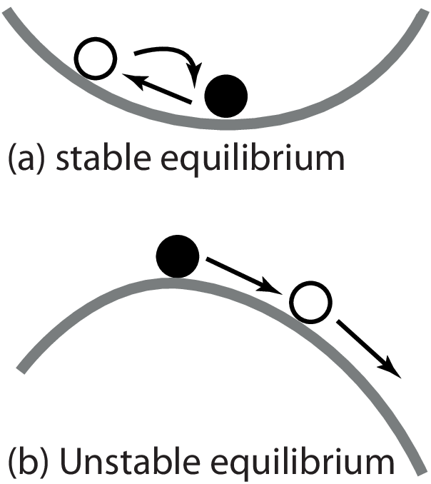 Equilibrium is when opposing forces or influences are balanced, if you did economics you probably recognise the equilibrium as the point where demand and supply are equal, the definition applies to that too as the forces of demand and supply are balanced at that point, Equilibrium is very prominent in economic theories, not only in demand and supply (there's a lot of examples of it in the economics section), it is also referred to as the steady state. In physics, it's when an object is at rest, isn't moving, and has zero acceleration. There's stable and unstable equilibrium. Stable equilibrium implies the object in equilibrium will converge back to the equilibrium if it is displaced a little, like a spring when extended, and unstable equilibrium implies that a little displacement induced will result in the divergence of the object, like a ball on top of a hill if pushed.(www.researchgate.net/figure/Stable-and-unstable-equilibria-In-a-stable-equilibrium-a-small-disturbance-caused-by_fig1_261758142)
...
Statistical Misconceptions and Misuses New
Last edited on January 2026
Statistical Misconceptions
Statistics has been the backbone of decision-making throughout history, not used only by governments, research facilities, and big corporations, but also by us as individuals. Before you buy a product, statistics like the rating of the product on the internet and phrases like "Recommended by 90% of experts” can sway your decision to buy the product. Before you choose which university to go to, statistics like “100% of people who graduate from this institution are employed” , and “there is only a 50% chance of completing this degree in record time” , can also influence your decision. But in many cases, phrases like these, when looked at face value, can be misleading at best and outright false at worst. As such, it is very crucial to understand the statistical traps, we as people are prone to fall for. Interpreting data and statistics accurately is the first step towards making informed decisions. In this section, we will discuss 12 of those statistical traps.
1. Correlation ≠ Causation
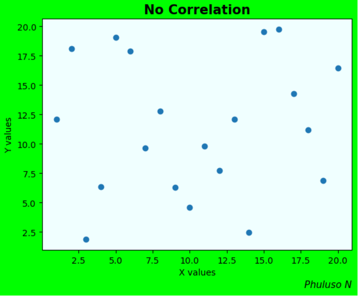
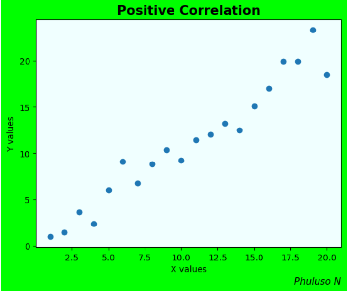
Correlation shows how strongly related 2 values are; in statistics, it is expressed numerically by the correlation coefficient(r). A positive correlation means that 2 values increase and decrease at the same time, and a negative correlation means that when one variable is increasing, the other is decreasing and vice versa. However, just because 2 events are correlated, doesn’t mean one caused the other.
Example
One famous example is the positive correlation between ice cream sales and shark attacks. When ice cream sales are high, so are the shark attacks. But ice cream isn't the cause of sharks attacking people, or vice versa; a more rational conclusion would be that it’s because more people buy ice cream, and more people go to the beach when it’s hot.
2. Sampling Bias or Selection Bias
Samplingis the process of selecting a smaller group as a representation of a larger group . This makes gathering data and making inferences about an entire group a lot simpler. Sampling bias, on the other hand, occurs when certain members of the group are more likely to be selected than others . This often leads to false inferences about the larger group due to the data being unfairly skewed.
What leads to sampling bias is when researchers use their judgment to select participants, when researchers select individuals or elements that are easiest to access or reach, flawed random selection methods, and when people with specific characteristics are more likely to agree to take part in a study than others.
Example
A One Piece social media fan page is doing a survey on what people think is the greatest manga, and the results come out as 99% for One Piece. Though One Piece is indeed the greatest, this is a form of sampling bias because the page is followed by mostly One Piece fans.
Sampling bias teaches how important it is to consider how a study was conducted and not just go with the percentage numbers alone.
3. Survivorship Bias
Survivorship bias is when we only assess the successful visible subgroup as the entire group.
Example 1
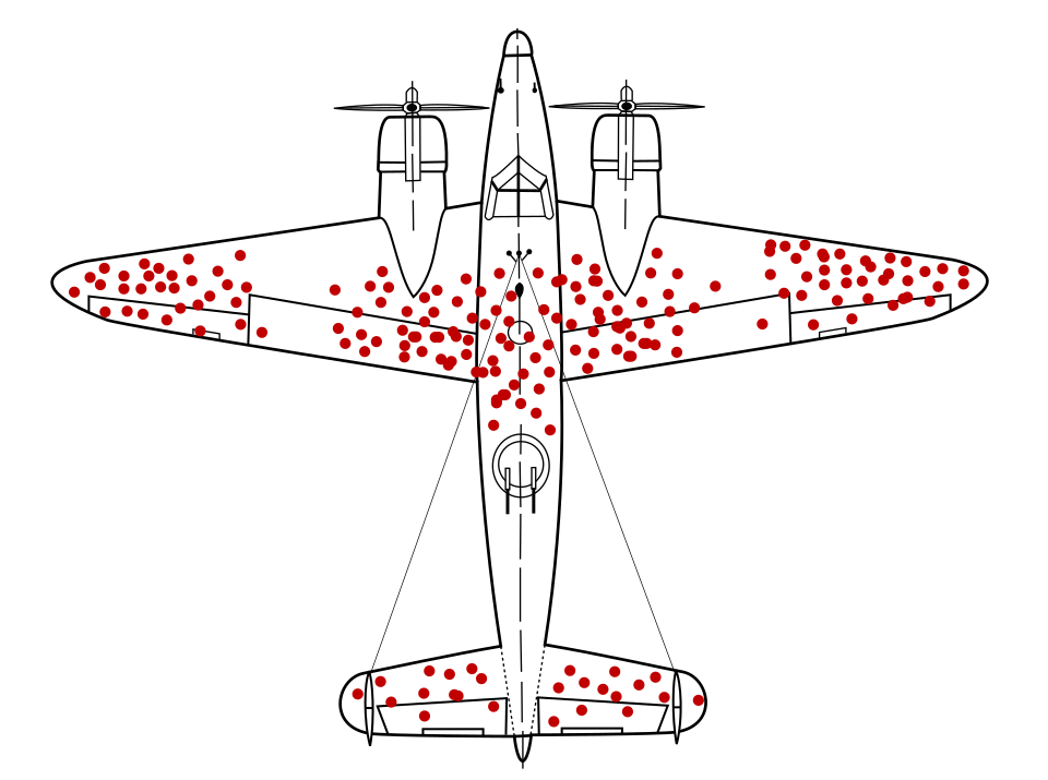
A famous example is from WW2, when a military research group was trying to figure out the locations to reinforce bomber planes for better protection, the first idea was to reinforce it based on the locations that the returning planes suffered the most damage, Abraham Wald, a famous statistician, noted that the most severely damaged planes were actually the ones that did not return. And that the locations on the returned planes were spots in which aircraft could sustain many bullet holes and still return, while the planes that sustained enemy fire in other locations were the ones that went down
Example 2
When people see old buildings that are still standing and conclude that people in the past were much better at architecture, while in reality, they’re just a few of the ones still standing out of many that were built.
Example 3
When we conclude that a certain career path is the best choice after seeing the successful people in that field and ignoring the thousands of others who failed.
4. False Causality Fallacies
A false cause fallacy occurs when someone falsely assumes that one thing caused another. The fallacy comes in many different forms, most notable ones being: Post Hoc Ergo Propter Hoc, Cum Hoc Ergo Propter Hoc and Non causa pro causa
Examples:
1. Post Hoc Ergo Propter Hoc, Latin for “after this, therefore because of this.”- Concluding that one event caused the other because one occurred after the other.
Example 1:
Phuluso buys a new study guide and gets better grades; therefore, buying the new study guide makes you get better grades.2. Cum Hoc Ergo Propter Hoc, Latin for “with this, therefore because of this.”- Concluding that one event caused the other because they occur at the same time
Example 1:
Phuluso listens to classical music while studying and gets good grades; therefore, listening to classical music while studying gets you better grades.Non causa pro causa, Latin for "not the cause for the cause."- Concluding that one event caused the other using insufficient evidence.
Example 1:
Phuluso has a medical aid, and he is always sick. Therefore, the medical aid is making him sick.5. Will Rogers paradox
Will Rogers paradox occurs when moving a data point from group 1 to group 2 raises the average of both groups.
Example
The poorest person in a rich country moves to a poor country where they’re now the richest in that country. The average of the rich country will go up because it lost a poor person in comparison, but the poor country’s average will also go up, because it gained a rich person in comparison. Both countries, on average, got richer, though no real improvement was actually made.
6. Regression Toward the Mean
Regression toward the mean is a statistical phenomenon that, if one variable is very high or very low on the first measurement, then it will tend toward the mean on its second measurement. Regression toward the mean is possible due to randomness. When you get an outlier when measuring a variable, it is often because other one-time random events were also at play, events that will not be at play when you measure the variable again. Hence, it will return closer to the mean.
Example 1
If a runner finishes a marathon in record time, in their next marathon, they’re likely going to finish in a longer time, a time that is closer to their average time. This is because peak performance is influenced by a variety of factors, including random factors that are not always present like luck. It’s possible they achieved the record because they had a well-rested sleep, ate the perfect breakfast, and did not have any stress that would affect their performance, the wind was in their favour, etc.
Example 2
If a student gets a very high score on a math test, in their next math test, they will likely get a lower score, closer to their average, even if they studied just as much as before, but because of reasons like the chapters they studied were not on the test, they didn't have enough sleep, and they were stressed when writing and other things outside their control.
Regression toward the mean fallacy
Regression toward the mean fallacy occurs when people attribute different reasons for things that happened due to a normal regression towards the mean. For example, The same student who got a high score on the previous test scored lower. the teacher might say it’s because the student did not study as much, when they did, just that odds were not in their favour this time around. or people might claim the athlete who finished in record-breaking time got arrogant and did worse in the next round, when that’s also not the case.
Such false attributions can lead to unnecessary policy or businesses model changes when companies and states don’t take Regression toward the mean into account when making statistically based decisions.
7. Hawthorne Effect or participant reactivity
Coined from a Harvard study conducted in 1924-1932, The Hawthorne effect is a phenomenon where people act differently when they are aware that they are being observed. As such, the observed behaviour may not represent the normal behaviour leading to wrong conclusions when conducting experiments.
Example 1
If you are conducting a study on whether workers are more productive in a cold or hot environment, chances are, if workers know they are being studied, they will work hard in both environments out of fear of appearing lazy.
8.Simpson's Paradox
Simpson's paradox occurs when groups of data show one trend, but this trend is reversed when the groups are combined.
Example
|
Male |
Female |
Acceptance per course |
|
|
Course 1 |
\(\frac{1712}{2744} = 62\%\) |
\(\frac{468}{588} = 80\%\) |
\(\frac{2180}{3332} = 65\%\) |
|
Course 2 |
\(\frac{676}{2638} = 26\%\) |
\(\frac{820}{3082} = 27\%\) |
\(\frac{1496}{5720} = 26\%\) |
|
Acceptance per gender |
\(\frac{2388}{5382} = 44\%\) |
\(\frac{1288}{3670} = 35\%\) |
Look at the diagram above. The total application acceptance of men is 44%, which is higher than the respective 35% for women. However, if we break things down by each course, you'll find that women scored higher than men in each course, 80% and 27% vs 62% and 26% for Courses 1 and 2 respectively. This is what is known as the Simpson's paradox, the skew is caused by the fact that more women applied a highly competitive course with with low acceptance rates for everyone. This is based on the UC Berkeley Gender Bias controversy (1973) where the university was accused of gender bias until the data was broken down by departments.
The Simpson's Paradox teaches us to look at data from every angle before making conclusions.
9. McNamara Fallacy
The McNamara Fallacy happens when you only focus on factors that can be numerically represented or measured, quantitative factors, while ignoring qualitative factors, those that cannot be accurately numerically represented or measured, which in many cases are just as important, if not more. Named after U.S. Secretary of Defence Robert McNamara, who relied heavily on easily quantifiable metrics, like enemy body counts, to measure success during the Vietnam War (1955-1975), ignoring crucial unquantifiable factors like the morale of the Vietnamese people and the political instability within the U.S., leading to a strategic failure despite the US having overall higher metrics in many categories.
Example 1
An ad campaign using the quantifiable number of YouTube video clicks to measure the success of an ad without taking into consideration that they probably clicked it by mistake, or how annoying the ad is to the customers and is damaging the brand reputation.
Example 2
Assessing a country’s prosperity by looking at Gross Domestic Product (GDP) alone, without taking into consideration the income distribution and overall well-being of the individual citizens.
10. Base rate fallacy (base rate neglect)
The Base rate fallacy Is a statistical fallacy where people ignore the base rate or original probability when making judgments about the likelihood of an event, it stems from failure to apply Bayes' theorem, a probability theorem which describes the probability of an event based on conditions that are related to the event. \(P(A \mid B) = \frac{P(B \mid A)\,P(A)}{P(B)}\).
Example
Suppose there are 100 students in a class, and 10 of them drink a Red Bull energy drink before studying for an exam. If you see a student pulling an all-nighter and assume they must be one of the Red Bull drinkers, then you have fallen for the base rate fallacy. Even if Red Bull drinkers are more likely to study all night, there are far more students who don’t drink it, so most all-nighters will still most likely come from the non-Red Bull drinking group.
11. Gambler's Fallacy
Suppose you have 10 blue balls and 5 red balls in a bag, without looking inside the bag, what is the probability of reaching inside and taking out a red ball? it’s \(5\over 15\) =33.33% because there are 5 red balls and a total of 15 balls. Now suppose you do take out the red ball, and now there are 4 red balls. Now, what is the probability of taking out the red ball again? \(5\over 15\)=26.66%, there is now a lower probability compared to the first attempt. This is because the first and second events of taking the ball out of the bag are dependent on each other; in probability, these are called dependent events.
Now, on the other hand, suppose you have a coin, and you flip it, what is the probability it will be heads? It's \(1 \over2\)=50%, and if you flip it again, after getting heads, what is the probability of getting heads again? still \(1 \over2\)=50%. This is because these 2 events are independent of each other, even if you flip the coin 10 times and get heads, the probability of getting heads the next time you flip is still the same.
Gambler's Fallacy
The Gambler's fallacy is the belief that because something has happened more frequently than usual, it’s now less likely to happen in the future, and vice versa. This stems from confusing independent events with dependent events.
Example
Suppose you flip the coin 50 times and it lands on heads, the next time you flip it, you will more than likely expect it to be tails , even though the probability is still the same.
12. Multiple comparisons fallacy (multiple testing problem)
Every statistical test or experiment is likely to contain some error or unexpected finding because nothing is perfect, as such, the more you make conduct tests, the more errors you’re likely to run into. The multiple comparisons fallacy occurs when researchers take such errors to be significant findings, even though they appeared by chance and are very few compared to the rest of the findings
Example
Suppose you run 20 different tests to determine whether a lotion is effective. By chance alone, one person’s condition improves, and you then claim the lotion is effective. This is the multiple comparisons fallacy, because when many tests are performed, some positive or negative results are expected to occur purely by chance.
Bibliography
- Gescheider, G.A., 2013. Psychophysics: the fundamentals. Psychology Press.
- Wixted, J.T. and Ebbesen, E.B., 1991. In the form of forgetting. Psychological science, 2(6), pp.409-415.
- Gottman, J., Swanson, C. and Murray, J., 1999. The mathematics of marital conflict: Dynamic mathematical nonlinear modeling of newlywed marital interaction. Journal of Family Psychology, 13(1), p.3.
- Ashby, N., 2003. Relativity in the global positioning system. Living Reviews in relativity, 6(1), pp.1-42.
- Black, D., 1948. On the rationale of group decision-making. Journal of political economy, 56(1), pp.23-34.
- Dunlap, R.A., 1997. The golden ratio and Fibonacci numbers. World Scientific.
- Bains, R., 1990. Fundamentals of Mathematical Analysis: Edited by Rod Haggarty Addison-Wesley Publishing Company 1989, 268 pp., ISBN: 0-201-41636-0.
- Haigh, T., Priestley, P.M. and Rope, C., 2016. ENIAC in action: Making and remaking the modern computer. MIT press.
- Barro, R.J. and Sala-i-Martin, X., 1992. Convergence. Journal of Political Economy, 100(2), pp.223-251.
- Riley, J.G., 1979. Informational equilibrium. Econometrica: Journal of the Econometric Society, pp.331-359.
- Barrowman, N., 2014. Correlation, causation, and confusion. The New Atlantis, pp.23-44.
- Feinstein, A.R., Sosin, D.M. and Wells, C.K., 1985. The Will Rogers phenomenon: stage migration and new diagnostic techniques as a source of misleading statistics for survival in cancer. New England Journal of Medicine, 312(25), pp.1604-1608.
- Rubin, M., 2024. Inconsistent multiple testing corrections: The fallacy of using family-based error rates to make inferences about individual hypotheses. Methods in Psychology, 10, p.100140.
- Clotfelter, C.T. and Cook, P.J., 1993. The “gambler's fallacy” in lottery play. Management Science, 39(12), pp.1521-1525.
- Bar-Hillel, M., 1980. The base-rate fallacy in probability judgments. Acta Psychologica, 44(3), pp.211-233.
- Jannach, D. and Bauer, C., 2020. Escaping the McNamara fallacy: Towards more impactful recommender systems research. Ai Magazine, 41(4), pp.79-95
- Oswald, D., Sherratt, F. and Smith, S., 2014. Handling the Hawthorne effect: The challenges surrounding a participant observer. Review of social studies, 1(1), pp.53-73.
- Pinto, R., 2001. Argument, inference and dialectic: Collected papers on informal logic (Vol. 4). Springer Science & Business Media.
- Elston, D.M., 2021. Survivorship bias. Journal of the American Academy of Dermatology
- Barnett, A.G., Van Der Pols, J.C. and Dobson, A.J., 2005. Regression to the mean: what it is and how to deal with it. International journal of epidemiology, 34(1), pp.215-220.
- Blyth, C.R., 1972. On Simpson's paradox and the sure-thing principle. Journal of the American Statistical Association, 67(338), pp.364-366.